内容目录
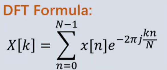
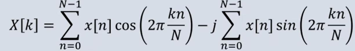
公式
demo1
import numpy as np
import matplotlib.pyplot as plt

# 离散时间傅里叶变换函数
def dft1(xx):
    # 生成时间序列
    t = np.linspace(0, 1.0, len(xx))
    # 初始化频率数组
    f = np.arange(len(xx) // 2 + 1, dtype=complex)
    # 计算傅里叶变换
    for index in range(len(f)):
        # 计算频率 index 对应的复数值
        f[index] = complex(np.sum(np.cos(2 * np.pi * index * t) * xx), -np.sum(np.sin(2 * np.pi * index * t) * xx))
    return f

# 设置采样频率
sampling_rate = 1000
# 采样时间(单位s)
sampling_time = 20
t1 = np.arange(0, sampling_time, 1.0 / sampling_rate)
# 构造信号
x1 = np.sin(15 * np.pi * t1) + np.cos(6.5 * np.pi * t1) + np.cos(5 * np.pi * t1)

# 进行傅里叶变换并归一化
xf = dft1(x1) / len(x1)
# 计算频率
freqs = np.linspace(0, sampling_rate, int(len(x1) / 2 + 1))

absxf = 2 * np.abs(xf)
# 找出大于1的值的索引
indices = np.where(absxf > 0.5)[0]
print("频率", indices * 2 / sampling_time)

# 绘制傅里叶变换结果的幅频特性曲线
plt.figure(figsize=(16, 4))
plt.plot(freqs, 2 * np.abs(xf), 'r--')

plt.xlabel("Frequency(Hz)")
plt.ylabel("Amplitude($m$)")
plt.title("Amplitude-Frequency curve")

plt.show()

# 绘制截取频率范围内的幅频特性曲线
plt.figure(figsize=(16, 4))
plt.plot(freqs, 2 * np.abs(xf), 'r--')

plt.xlabel("Frequency(Hz)")
plt.ylabel("Amplitude($m$)")
plt.title("Amplitude-Frequency curve")
plt.xlim(0, 20)  # 截取频率范围

plt.show()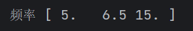
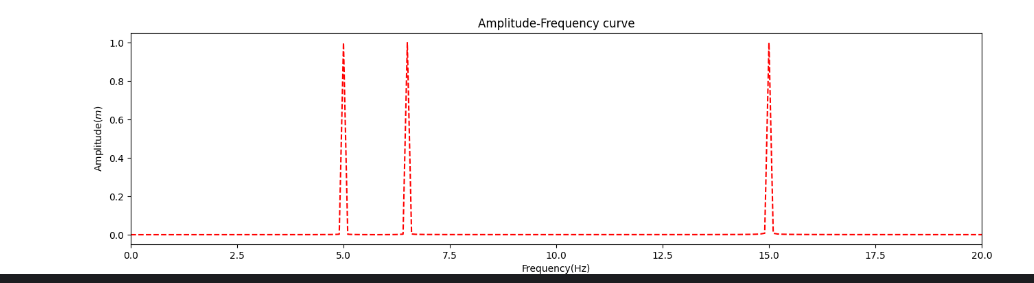
可以正确找出频率
demo2
absxf = 2 * np.abs(xf)
# 找出大于1的值的索引
indices = np.where(absxf > 0.5)[0]
print("频率", indices * 2 / sampling_time)
for i in indices:
temp = xf[i]
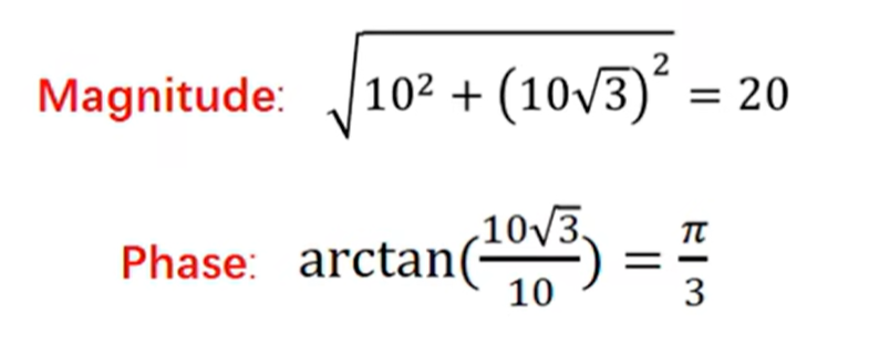
magnitude = math.sqrt(temp.real * temp.real + temp.imag * temp.imag)
phase = np.arctan(temp.imag / temp.real)
print("fre", i * 2 / sampling_time, "mag", magnitude, "phase", phase)通过上述代码,能够找到傅里叶转换后的cos函数对应的频率、幅值、相位
x1 = 2 * np.cos(5 * np.pi * t1) + np.cos(6.5 * np.pi * t1 - 1) + np.cos(15 * np.pi * t1)
fre 5.0 mag 0.9999693059786717 phase -0.00777369902672848
fre 6.5 mag 0.5001106976971383 phase -1.0097934293468178
fre 15.0 mag 0.5001119446975573 phase -0.023599666703126954
可见 $(mag/0.5) cos(fre \pi * t + phase)$
import math

import numpy as np
import matplotlib.pyplot as plt

# 离散时间傅里叶变换函数
def dft1(xx):
    # 生成时间序列
    t = np.linspace(0, 1.0, len(xx))
    # 初始化频率数组
    f = np.arange(len(xx) // 2 + 1, dtype=complex)
    # 计算傅里叶变换
    for index in range(len(f)):
        # 计算频率 index 对应的复数值
        f[index] = complex(np.sum(np.cos(2 * np.pi * index * t) * xx), -np.sum(np.sin(2 * np.pi * index * t) * xx))
    return f

# 设置采样频率
sampling_rate = 1000
# 采样时间(单位s)
sampling_time = 20
t1 = np.arange(0, sampling_time, 1.0 / sampling_rate)
# 构造信号
x1 = 2 * np.cos(5 * np.pi * t1) + np.cos(6.5 * np.pi * t1 - 1) + np.cos(15 * np.pi * t1)

# 进行傅里叶变换并归一化
xf = dft1(x1) / len(x1)

# 计算频率
freqs = np.linspace(0, sampling_rate, int(len(x1) / 2 + 1))

absxf = 2 * np.abs(xf)
# 找出大于1的值的索引
indices = np.where(absxf > 0.5)[0]
for i in indices:
    temp = xf[i]
    magnitude = math.sqrt(temp.real * temp.real + temp.imag * temp.imag)
    phase = np.arctan(temp.imag / temp.real)
    print("fre", i * 2 / sampling_time, "mag", magnitude, "phase", phase)

# 绘制傅里叶变换结果的幅频特性曲线
plt.figure(figsize=(16, 4))
plt.plot(freqs, 2 * np.abs(xf), 'r--')

plt.xlabel("Frequency(Hz)")
plt.ylabel("Amplitude($m$)")
plt.title("Amplitude-Frequency curve")

plt.show()

# 绘制截取频率范围内的幅频特性曲线
plt.figure(figsize=(16, 4))
plt.plot(freqs, 2 * np.abs(xf), 'r--')

plt.xlabel("Frequency(Hz)")
plt.ylabel("Amplitude($m$)")
plt.title("Amplitude-Frequency curve")
plt.xlim(0, 20)  # 截取频率范围

plt.show()
封装
# 传入dft1函数返回的对象除以dft1函数的输入的长度,即xf = dft1(x1) / len(x1)。sampling_time即采样时间
def getcos(xf, sampling_time):
    results = []
    absxf = 2 * np.abs(xf)
    # 找出大于1的值的索引
    indices = np.where(absxf > 0.5)[0]
    for i in indices:
        temp = xf[i]
        magnitude = math.sqrt(temp.real * temp.real + temp.imag * temp.imag)
        phase = np.arctan(temp.imag / temp.real)
        results.append({'magnitude': magnitude, 'phase': phase, 'temp': temp})
        print("fre", i * 2 / sampling_time, "mag", magnitude, "phase", phase)
    return results
应用:去除工频噪声
import math

import numpy as np
import matplotlib.pyplot as plt

# 离散时间傅里叶变换函数
def dft1(xx):
    # 生成时间序列
    t = np.linspace(0, 1.0, len(xx))
    # 初始化频率数组
    f = np.arange(len(xx) // 2 + 1, dtype=complex)
    # 计算傅里叶变换
    for index in range(len(f)):
        # 计算频率 index 对应的复数值
        f[index] = complex(np.sum(np.cos(2 * np.pi * index * t) * xx), -np.sum(np.sin(2 * np.pi * index * t) * xx))
    return f

# 传入dft1函数返回的对象除以dft1函数的输入的长度,即xf = dft1(x1) / len(x1)。sampling_time即采样时间
def getcos(xf, sampling_time):
    results = []
    absxf = 2 * np.abs(xf)
    # 找出大于1的值的索引
    indices = np.where(absxf > 0.5)[0]
    for i in indices:
        temp = xf[i]
        magnitude = math.sqrt(temp.real * temp.real + temp.imag * temp.imag)
        phase = np.arctan(temp.imag / temp.real)
        results.append({'fre' : i, 'magnitude': magnitude, 'phase': phase})
        print("fre", i, "mag", magnitude, "phase", phase)
    return results

# 生成方波信号
T = 0.1  # 周期
sampling_rate = 1000  # 采样率
sampling_time = 1
t = np.arange(0, 2, sampling_time/sampling_rate)  # 时间向量
duty_cycle = 0.5  # 占空比
square_wave = np.sign(np.sin(2 * np.pi * t / T))

# 生成工频噪声和高斯白噪声
freq_noise_amplitude = 2.5
gaussian_noise_std = 0.25
freq_noise = freq_noise_amplitude * np.cos(np.pi * 50 * t)  # 50Hz的工频噪声
gaussian_noise = np.random.normal(0, gaussian_noise_std, len(t))  # 高斯白噪声

# 叠加噪声到方波信号上
noisy_signal = square_wave + freq_noise + gaussian_noise

# 傅里叶
xf = dft1(noisy_signal - square_wave) / len(noisy_signal)
results = getcos(xf, sampling_time)
print(results)

# 去除噪声
for result in results:
    fre = result['fre']
    magnitude = result['magnitude']
    phase = result['phase']
    noise = (magnitude / 0.5) * np.cos(fre * np.pi * t + phase)
    noisy_signal = noisy_signal - noise
noisy_signal = np.sign(noisy_signal)

# 计算不匹配数量
mismatch_count = np.sum(noisy_signal != square_wave)
print("不匹配数量:", mismatch_count)
print("不匹配比例:", mismatch_count / square_wave.size)

freqs = np.linspace(0, sampling_rate, int(len(noisy_signal) / 2 + 1))

# 绘制截取频率范围内的幅频特性曲线
plt.figure(figsize=(16, 4))
plt.plot(freqs, 2 * np.abs(xf), 'r--')

plt.xlabel("Frequency(Hz)")
plt.ylabel("Amplitude($m$)")
plt.title("Amplitude-Frequency curve")
plt.xlim(0, 250)  # 截取频率范围
plt.show()

# 画图比较
plt.figure(1,figsize=(12, 6))
plt.subplot(2, 1, 1)
plt.plot(t, square_wave, label='Original Signal')
plt.plot(t, noisy_signal, 'r--', label='Filtered Signal')
plt.title('Before Filtering')
plt.xlabel('Time (s)')
plt.ylabel('Amplitude')
plt.legend()
plt.tight_layout()
plt.show()
[[噪声去除]]